Der Verbund simplizialer Mengen ist im mathematischen Teilgebiet der Höheren Kategorietheorie eine Operation, welche die Kategorie der simplizialen Mengen zu einer monoidalen Kategorie macht. Insbesondere macht der Verbund aus zwei simplizialen Mengen eine weitere simplizialen Menge. Darüber ist der Verbund simplizialer Mengen verwandt mit der Diamantoperation und wird bei der Konstruktion der getwisteten Diagonale verwendet. Unter dem Nerv korrespondiert der Verbund simplizialer Mengen mit dem Verbund kleiner Kategorien und unter der geometrischen Realisierung zum Verbund topologischer Räume .
Definition
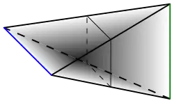
Visualisierung des Verbundes
X
∗
Y
{\displaystyle X*Y}
X
{\displaystyle X}
Y
{\displaystyle Y}
Für natürliche Zahlen
m
,
p
,
q
∈
N
{\displaystyle m,p,q\in \mathbb {N} }
[ 1]
Hom
(
[
m
]
,
[
p
+
q
+
1
]
)
=
∏
i
+
j
+
1
=
n
Hom
(
[
i
]
,
[
p
]
)
×
Hom
(
[
j
]
,
[
q
]
)
,
{\displaystyle \operatorname {Hom} ([m],[p+q+1])=\prod _{i+j+1=n}\operatorname {Hom} ([i],[p])\times \operatorname {Hom} ([j],[q]),}
welcher durch Kolimiten zu einem Funktor
−
∗
−
:
s
S
e
t
×
s
S
e
t
→
s
S
e
t
{\displaystyle -*-\colon \mathbf {sSet} \times \mathbf {sSet} \rightarrow \mathbf {sSet} }
s
S
e
t
{\displaystyle \mathbf {sSet} }
monoidalen Kategorie macht. Für simpliziale Mengen
X
{\displaystyle X}
Y
{\displaystyle Y}
X
∗
Y
{\displaystyle X*Y}
[ 2] [ 3] [ 1]
(
X
∗
Y
)
n
=
∏
i
+
j
+
1
=
n
X
i
×
Y
j
.
{\displaystyle (X*Y)_{n}=\prod _{i+j+1=n}X_{i}\times Y_{j}.}
Ein
n
{\displaystyle n}
σ
:
Δ
n
→
X
∗
Y
{\displaystyle \sigma \colon \Delta ^{n}\rightarrow X*Y}
X
{\displaystyle X}
Y
{\displaystyle Y}
p
{\displaystyle p}
σ
−
:
Δ
p
→
X
{\displaystyle \sigma _{-}\colon \Delta ^{p}\rightarrow X}
q
{\displaystyle q}
σ
+
:
Δ
q
→
Y
{\displaystyle \sigma _{+}\colon \Delta ^{q}\rightarrow Y}
n
=
p
+
q
+
1
{\displaystyle n=p+q+1}
σ
=
σ
−
∗
σ
+
{\displaystyle \sigma =\sigma _{-}*\sigma _{+}}
[ 4]
Es gibt kanonische Morphismen
X
,
Y
→
X
∗
Y
{\displaystyle X,Y\rightarrow X*Y}
X
+
Y
→
X
∗
Y
{\displaystyle X+Y\rightarrow X*Y}
X
∗
Y
→
Δ
0
∗
Δ
0
≅
Δ
1
{\displaystyle X*Y\rightarrow \Delta ^{0}*\Delta ^{0}\cong \Delta ^{1}}
0
{\displaystyle 0}
X
{\displaystyle X}
1
{\displaystyle 1}
Y
{\displaystyle Y}
Für eine simpliziale Menge
X
{\displaystyle X}
linker und rechter Kegel definiert als:
X
◃
:=
Δ
0
∗
X
;
{\displaystyle X^{\triangleleft }:=\Delta ^{0}*X;}
X
▹
:=
X
∗
Δ
0
.
{\displaystyle X^{\triangleright }:=X*\Delta ^{0}.}
Rechtsadjungierte
Sei
Y
{\displaystyle Y}
Y
∗
−
:
s
S
e
t
→
Y
∖
s
S
e
t
,
X
↦
(
Y
↦
Y
∗
X
)
{\displaystyle Y*-\colon \mathbf {sSet} \rightarrow Y\backslash \mathbf {sSet} ,X\mapsto (Y\mapsto Y*X)}
Rechtsadjungierten
Y
∖
s
S
e
t
→
s
S
e
t
,
(
t
:
Y
→
W
)
↦
t
∖
W
{\displaystyle Y\backslash \mathbf {sSet} \rightarrow \mathbf {sSet} ,(t\colon Y\rightarrow W)\mapsto t\backslash W}
Y
∖
W
{\displaystyle Y\backslash W}
−
∗
Y
:
s
S
e
t
→
Y
∖
s
S
e
t
,
X
↦
(
Y
↦
X
∗
Y
)
{\displaystyle -*Y\colon \mathbf {sSet} \rightarrow Y\backslash \mathbf {sSet} ,X\mapsto (Y\mapsto X*Y)}
Y
∖
s
S
e
t
→
s
S
e
t
,
(
t
:
Y
→
W
)
↦
W
/
t
{\displaystyle Y\backslash \mathbf {sSet} \rightarrow \mathbf {sSet} ,(t\colon Y\rightarrow W)\mapsto W/t}
W
/
Y
{\displaystyle W/Y}
[ 5] [ 6] [ 7] terminale simplizale Menge
Y
=
Δ
0
{\displaystyle Y=\Delta ^{0}}
s
S
e
t
∗
=
Δ
0
∖
s
S
e
t
{\displaystyle \mathbf {sSet} _{*}=\Delta ^{0}\backslash \mathbf {sSet} }
Sei
C
{\displaystyle {\mathcal {C}}}
X
∈
Ob
C
{\displaystyle X\in \operatorname {Ob} {\mathcal {C}}}
[
0
]
{\displaystyle [0]}
terminale Kategorie (wobei die Notation vom terminalen Objekt der Simplexkategorie stammt), dann gibt es einen assoziierten Funktor
t
:
[
0
]
→
C
,
0
↦
X
{\displaystyle t\colon [0]\rightarrow {\mathcal {C}},0\mapsto X}
N
t
:
Δ
0
→
N
C
{\displaystyle Nt\colon \Delta ^{0}\rightarrow N{\mathcal {C}}}
A
{\displaystyle A}
[ 8]
s
S
e
t
(
A
,
N
C
/
N
t
)
≅
s
S
e
t
∗
(
Δ
0
→
A
∗
Δ
0
,
N
t
)
≅
C
a
t
∗
(
[
0
]
→
τ
(
A
)
⋆
[
0
]
,
t
)
≅
C
a
t
(
τ
(
A
)
,
C
/
X
)
≅
s
S
e
t
(
A
,
N
(
C
/
X
)
)
.
{\displaystyle {\begin{aligned}\mathbf {sSet} (A,N{\mathcal {C}}/Nt)&\cong \mathbf {sSet} _{*}(\Delta ^{0}\rightarrow A*\Delta ^{0},Nt)\cong \mathbf {Cat} _{*}([0]\rightarrow \tau (A)\star [0],t)\\&\cong \mathbf {Cat} (\tau (A),{\mathcal {C}}/X)\cong \mathbf {sSet} (A,N({\mathcal {C}}/X)).\end{aligned}}}
Nach dem Lemma von Yoneda gilt daher (mit der alternativen Notation zur Betonung des Resultates):[ 9] [ 7]
N
C
/
N
X
≅
N
(
C
/
X
)
.
{\displaystyle N{\mathcal {C}}/NX\cong N({\mathcal {C}}/X).}
Beispiele
Es gilt:[ 10]
∂
Δ
m
∗
Δ
n
∪
Δ
m
∗
∂
Δ
n
≅
∂
Δ
m
+
n
+
1
,
{\displaystyle \partial \Delta ^{m}*\Delta ^{n}\cup \Delta ^{m}*\partial \Delta ^{n}\cong \partial \Delta ^{m+n+1},}
Λ
k
m
∗
Δ
n
∪
Δ
m
∗
∂
Δ
n
≅
Λ
k
m
+
n
+
1
,
{\displaystyle \Lambda _{k}^{m}*\Delta ^{n}\cup \Delta ^{m}*\partial \Delta ^{n}\cong \Lambda _{k}^{m+n+1},}
∂
Δ
m
∗
Δ
n
∪
Δ
m
∗
Λ
k
n
≅
Λ
m
+
k
+
1
m
+
n
+
1
.
{\displaystyle \partial \Delta ^{m}*\Delta ^{n}\cup \Delta ^{m}*\Lambda _{k}^{n}\cong \Lambda _{m+k+1}^{m+n+1}.}
Eigenschaften
Für simpliziale Mengen
X
{\displaystyle X}
Y
{\displaystyle Y}
γ
X
,
Y
:
X
⋄
Y
→
X
∗
Y
{\displaystyle \gamma _{X,Y}\colon X\diamond Y\rightarrow X*Y}
Diamantoperation , welcher mit den kanonischen Morphismen
X
+
Y
→
X
∗
Y
,
X
⋄
Y
{\displaystyle X+Y\rightarrow X*Y,X\diamond Y}
X
∗
Y
,
X
⋄
Y
→
Δ
1
{\displaystyle X*Y,X\diamond Y\rightarrow \Delta ^{1}}
[ 11] Joyal-Modellstruktur .[ 12] [ 13]
Für eine simpliziale Menge
X
{\displaystyle X}
X
∗
−
,
−
∗
X
:
s
S
e
t
→
s
S
e
t
{\displaystyle X*-,-*X\colon \mathbf {sSet} \rightarrow \mathbf {sSet} }
[ 14]
Für ∞-Kategorien
X
{\displaystyle X}
Y
{\displaystyle Y}
X
∗
Y
{\displaystyle X*Y}
[ 15] [ 16]
Der Verbund ist assoziativ. Für simpliziale Mengen
X
{\displaystyle X}
Y
{\displaystyle Y}
Z
{\displaystyle Z}
(
X
∗
Y
)
∗
Z
≅
X
∗
(
Y
∗
Z
)
.
{\displaystyle (X*Y)*Z\cong X*(Y*Z).}
Der Verbund kehrt sich unter der dualen simplizialen Menge um. Für simpliziale Mengen
X
{\displaystyle X}
Y
{\displaystyle Y}
[ 17] [ 18]
(
X
∗
Y
)
o
p
≅
Y
o
p
∗
X
o
p
.
{\displaystyle (X*Y)^{\mathrm {op} }\cong Y^{\mathrm {op} }*X^{\mathrm {op} }.}
Für einen Morphismus
t
:
Y
→
W
{\displaystyle t\colon Y\rightarrow W}
[ 18]
(
W
/
t
)
o
p
≅
t
o
p
∖
W
o
p
.
{\displaystyle (W/t)^{\mathrm {op} }\cong t^{\mathrm {op} }\backslash W^{\mathrm {op} }.}
Für einen Morphismus
z
:
Y
∗
X
→
W
{\displaystyle z\colon Y*X\rightarrow W}
x
:
X
→
Y
∗
X
→
W
{\displaystyle x\colon X\rightarrow Y*X\rightarrow W}
y
:
Y
→
W
/
x
{\displaystyle y\colon Y\rightarrow W/x}
z
{\displaystyle z}
s
S
e
t
(
Y
,
W
/
x
)
≅
X
∖
s
S
e
t
(
X
→
Y
∗
X
,
x
)
{\displaystyle \mathbf {sSet} (Y,W/x)\cong X\backslash \mathbf {sSet} (X\rightarrow Y*X,x)}
W
/
z
≅
(
W
/
x
)
/
y
{\displaystyle W/z\cong (W/x)/y}
[ 18]
W
/
(
Y
∗
X
)
≅
(
W
/
X
)
/
Y
.
{\displaystyle W/(Y*X)\cong (W/X)/Y.}
Beweis: Für jede simpliziale Menge
A
{\displaystyle A}
s
S
e
t
(
A
,
W
/
z
)
≅
(
Y
∗
X
)
∖
s
S
e
t
(
(
Y
∗
X
)
→
A
∗
(
Y
∗
X
)
,
z
)
≅
X
∖
s
S
e
t
(
X
→
(
A
∗
Y
)
∗
X
,
x
)
≅
s
S
e
t
(
A
∗
Y
,
W
/
x
)
≅
Y
∖
s
S
e
t
(
Y
→
A
∗
Y
,
y
)
≅
s
S
e
t
(
A
,
(
W
/
x
)
/
y
)
,
{\displaystyle {\begin{aligned}\mathbf {sSet} (A,W/z)&\cong (Y*X)\backslash \mathbf {sSet} ((Y*X)\rightarrow A*(Y*X),z)\cong X\backslash \mathbf {sSet} (X\rightarrow (A*Y)*X,x)\\&\cong \mathbf {sSet} (A*Y,W/x)\cong Y\backslash \mathbf {sSet} (Y\rightarrow A*Y,y)\cong \mathbf {sSet} (A,(W/x)/y),\end{aligned}}}
womit die Behauptung aus dem Lemma von Yoneda folgt.
Unter dem Nerv wird der Verbund kleiner Kategorien zum Verbund simplizialer Mengen. Für kleine Kategorien
C
{\displaystyle {\mathcal {C}}}
D
{\displaystyle {\mathcal {D}}}
[ 19] [ 20]
N
(
C
⋆
D
)
≅
N
C
∗
N
D
.
{\displaystyle N({\mathcal {C}}\star {\mathcal {D}})\cong N{\mathcal {C}}*N{\mathcal {D}}.}
Weblinks
Literatur
Einzelnachweise
↑ a b Cisinski 2019, 3.4.12.
↑ Joyal 2008, Proposition 3.1.
↑ Lurie 2009, Definition 1.2.8.1.
↑ Kerodon, Remark 4.3.3.17.
↑ Joyal 2008, Proposition 3.12.
↑ Lurie 2009, Proposition 1.2.9.2
↑ a b Cisinski 2019, 3.4.14.
↑ Lurie 2009, 1.2.9 Overcategories and Undercategories
↑ Joyal 2008, Proposition 3.13.
↑ Cisinski 2019, Proposition 3.4.17.
↑ Cisinski 2019, Proposition 4.2.2.
↑ Lurie 2009, Proposition 4.2.1.2.
↑ Cisinksi 2019, Proposition 4.2.3.
↑ Cisinski 2019, Corollary 4.2.5.
↑ Joyal 2008, Corollary 3.23.
↑ Lurie 2009, Proposition 1.2.8.3
↑ Joyal 2008, p. 244
↑ a b c Cisinski 2019, Remark 3.4.15.
↑ Joyal 2008, Corollary 3.3.
↑ Kerodon, Example 4.3.3.14.


![{\displaystyle \operatorname {Hom} ([m],[p+q+1])=\prod _{i+j+1=n}\operatorname {Hom} ([i],[p])\times \operatorname {Hom} ([j],[q]),}](./ebf7fb5ffe8d8cf89fe1bd828ba0aa1b401e94d8.svg)


![{\displaystyle [0]}](./ee314d016dd522b7f685325ca45f5e5003081fd0.svg)
![{\displaystyle t\colon [0]\rightarrow {\mathcal {C}},0\mapsto X}](./41097fad01f63c2b97761eeb5361b4a141339b2c.svg)


![{\displaystyle {\begin{aligned}\mathbf {sSet} (A,N{\mathcal {C}}/Nt)&\cong \mathbf {sSet} _{*}(\Delta ^{0}\rightarrow A*\Delta ^{0},Nt)\cong \mathbf {Cat} _{*}([0]\rightarrow \tau (A)\star [0],t)\\&\cong \mathbf {Cat} (\tau (A),{\mathcal {C}}/X)\cong \mathbf {sSet} (A,N({\mathcal {C}}/X)).\end{aligned}}}](./5356e9fba03855289e8c1875356ffae1fe3a1f60.svg)


